STA441 Assignment 11
Quiz in Tutorial on Thursday March 31st
For this assignment, our main analyses will be based on fixed effects models using proc mixed. The model is linear regression, possibly with dummy variables:
Yi = β0 + β1xi1 + β2xi2 + ... + βpxip + εi,
where the error terms εi are normally distributed with expected value zero. Error terms for the same case have a covariance matrix Σ. The matrix Σ could be have all σ2 values on the main diagonal and zeros on the off-diagonals. In this case we have ordinary regression with independent errors.
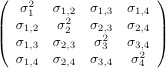
Quite a few other structures are available for Σ, including the following:
| Unknown (type=un) |
|
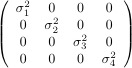
Variance Components (type=vc) |
|
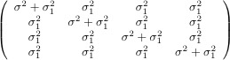
Compound Symmetry (type=cs) |
|
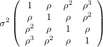
Autoregressive (type=ar(1)) |
 |
|
 |
|
 |
|
 |
These formulas will be provided with the last quiz, and they will be on the formula sheet for the final exam. For any set of proc mixed output you generate, you should be able to
- Give p, the number of explanatory variables in the regression model.
- Give the dimension (number of rows and columns) in Σ.
- Give the total number of parameters in the model you fit. That's the number of β values plus the number of unique elements in Σ.
- Locate any parameter estimates on your printout.
- For every test (and there may quite a few) be able to state the null hypothesis in terms of the symbols of your model.
- In a test of how well people remember instructional materials, subjects of various educational levels were presented with training materials that were either in Black & White or in Colour. Their ability to recall the material was tested with both Cartoon and Realistic testing materials at two points in time -- immediately after training, and several weeks later. Scores on an IQ test (the Otis Mental Ability Test) were available for all subjects. The variables are
- Subject identification number
- Colour of training materials: 0 = Black & White, 1 = Colour
- Education: 0 = Pre-professional, 1 = Professional, 2 = Student.
- Location: 1 = Hospital A, 2 = Hospital B, 3 = Hospital C, 4 = Penn State University.
- Otis Test of Mental Ability (IQ)
- Recall at Time One, Cartoon testing materials
- Recall at Time One, Realistic testing materials
- Recall at Time Two, Cartoon testing materials
- Recall at Time Two, Realistic testing materials
The data are available in the file
cartoon.data.txt. This is a Minitab data set.
- We will limit the analysis to students, who are all from Penn State University. I used an if statement, but I had to put if before output.This leaves us with a three-factor analysis of covariance.
- What is the covariate?
- What are the factors?
- Label each factor as within-cases or between-cases.
- Write the full regression model, with products of dummy variables for all possible interactions. I get 9 βs.
- Give the dimension (number of rows and columns) in Σ.
- Let's not assume anything about the structure of the covariance matrix. How many unique elements are there in Σ?
- Carry out the analysis using proc mixed. Just so you can see if we are on the same page, my -2 Restricted Log Likelihood was 878.6.
- For each F-test, be able to state the null hypothesis in Greek letters.
- Locate the estimate of each element of Σ on your printout. Don't bother with the β-hats.
- For each significant F-test, be able to state the conclusion in plain, non-statistical language. This will require some lsmeans.
- What is the null hypothesis for the "Null Model Likelihood Ratio Test?" Why does it have 9 degrees of freedom?
- This question uses data from the Toronto Raptors' 2006-2007 season. For
each regular season and playoff game, the following variables were recorded:
- Date
- Home or Away game
- Opponent
- Won or lost
- Days since last game (If I've made a mistake and you notice please let me know, but don't correct it.)
- Points scored by the Raptors
- Points scored by opponents
- Opponents' won-lost record the preceding year.
The data are available in the file
Raptors06-07.data.txt.
The response variable will be point spread, defined as Raptors' score
minus opponents' score. The explanatory variables will be Opponents' won-lost record, Home vs Away game, Days since last game, and a binary variable that equals one if the game was on a weekend, and zero if on a weekday.
Here a few hints and reminders intended to make it easier for you to read and process the data.
An ordinary regression on these data lacks all credibility, because it's obviously a time series and the assumption of independent random sampling (which means no sequential association between observations) is implausible without further evidence. So please follow these steps:
- Start with an ordinary regression, using the explanatory and response variables described above. Request the Durbin-Watson statistic, and save the residuals. So you can check, my regression had R2=0.2739.
- To see if the Durbin-Watson test is significant, you'll need the
Table. Take a look. How do you know that the test is inconclusive?
- Using proc arima, examine the autocorrelation function of the residuals. The lag 1 autocorrelation (around 0.175) comes right to the edge of the 95% interval around zero. Again, it's inconclusive. There might be some autocorrelation. If so, it's no more than lag one.
- Finally, run your regression analysis again using proc mixed, specifying a first-order autoregressive error structure. Please include the cl option on the proc mixed statement to get confidence intervals for the covariance parameters, and the / solution option on the model statement so you get the β-hats. They are not quite what you got from proc reg, because the usual beta-hats are maximum likelihood estimates (as well as least-squares), while these are restricted maximum likelihood (REML).
- In my output, there are two ways to test whether that first-order autocorrelation is zero. Is there acceptable evidence of sequential correlation in the errors?
- Compare the significance tests from proc mixed to those you got from proc reg. Do your conclusions change? What are those conclusions? For example, how many points was it worth for the Raptors to be playing on their home court? What is the value of the test statistic, and so on.
In summary, my conclusion is that the ordinary regression on these time series data was fine, but we didn't know it in advance. We had to check.
Please bring BOTH your log files and BOTH your your results files to the quiz. As usual, answers to the paper-and-pencil questions are not to be handed in. They are just practice for the quiz. Please do not write anything on your printouts except your name and student number. It is okay to highlight the results file, but do not write interpretations on your results files, or cause them to appear in any way (including comment statements) on your log files.