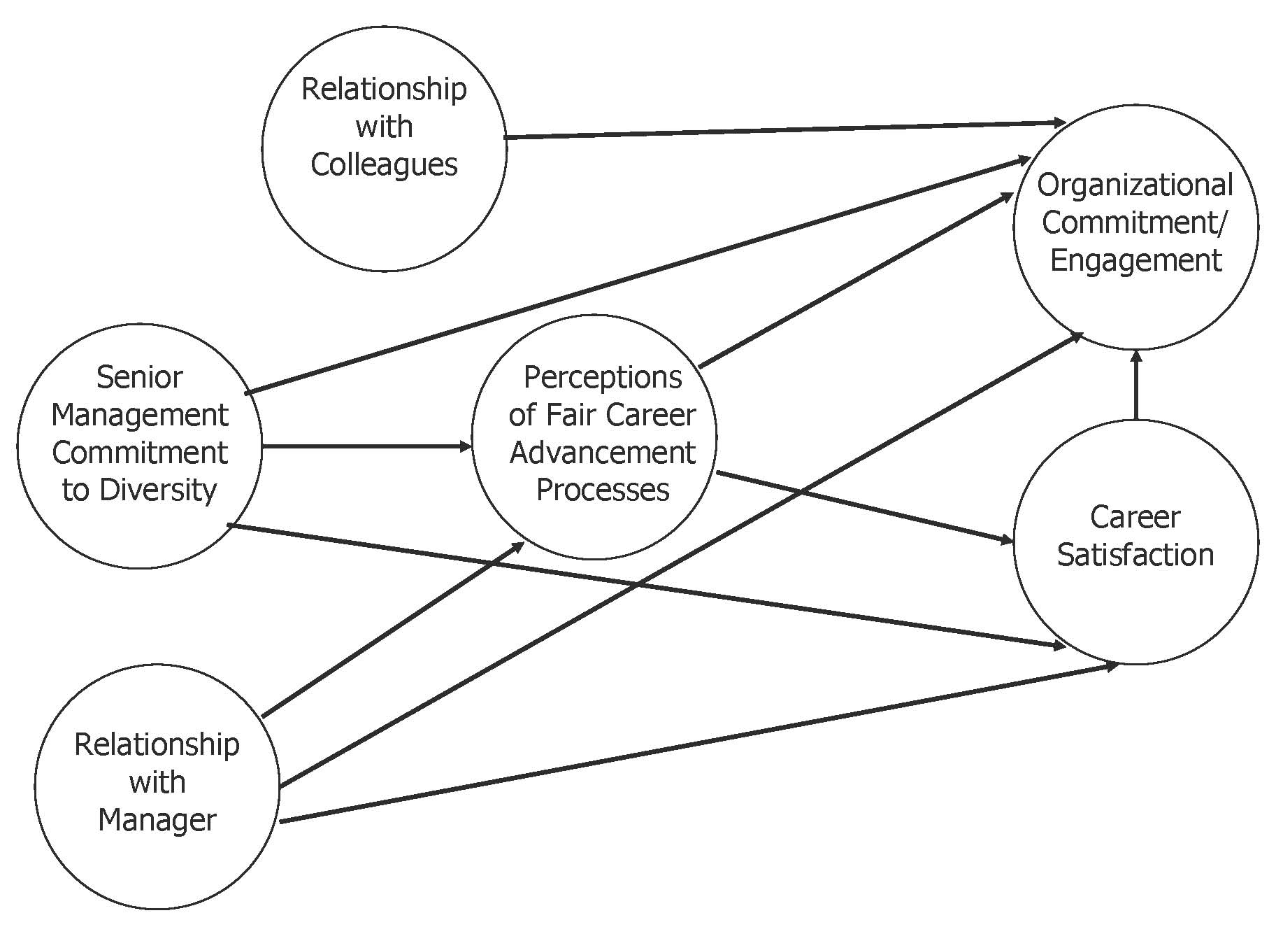
Diversity, Satisfaction and Organizational Commitment

| Relationship with Colleagues: | RelC1-RelC5 |
| Senior Management Commitment to Diversity: | SM1-SM3 |
| Relationship with Manager: | RelM1-RelM12 |
| Perceptions of Fair Career Advancement Processes: | Fair1-Fair6 |
| Career Satisfaction: | Sat1-Sat4 |
| Commitment to Organization: | Com1-Com10 |
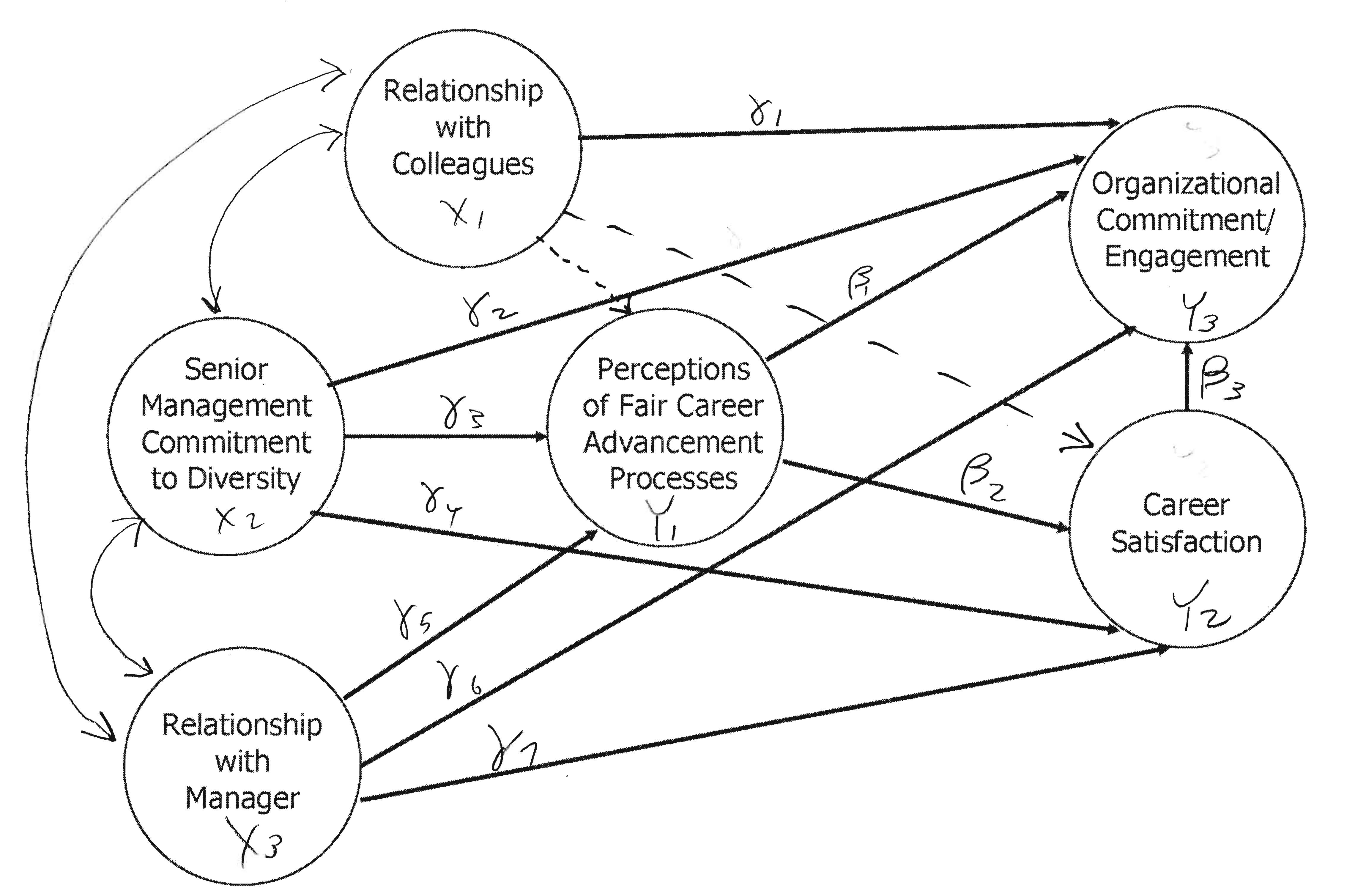

Data are in a spreadsheet.
/* diversity1.sas */
title 'Diversity study: Based on Catalyst (2007)';

/* Read data directly from Excel spreadsheet */
proc import datafile="/folders/myfolders/431s17/DiversityA.xls" out=HR dbms=xls;
            getnames=yes;
/* Input data file is DiversityA.xls
   Ouput data set is called HR (For Human Resources)
   dbms=xls The input file is an Excel spreadsheet.
            Necessary to read an Excel spreadsheet directly under unix/linux.
            Works in Windows environment too except for Excel 4.0 spreadsheets.
            The xlsx file type is supported, but as of SAS Version 9.3 it's flaky.
            If there are multiple sheets, use sheet="sheet1" or something.
   getnames=yes   Use column names as variable names                  */


proc contents;  /* See what's in there. */

proc format;  /* value labels used in data step below */
     value sexfmt  0 = 'Male'   1 = 'Female' ;
     value racefmt 0 = 'White'   1 = 'Visible Minority' ;

data diverse;
     set HR;
     commit1 = sum(of Com1-Com5);
     commit2 = sum(of Com6-Com10);
     commit = commit1+commit2;
     relcoll1 = RelC1+RelC2+RelC3;
     relcoll2 = RelC4+RelC5;
     relcol = relcoll1+relcoll2;
     relman1  = sum(of RelM1-RelM6);
     relman2  = sum(of RelM7-RelM12);
     relman = relman1+relman2;
     fairad1  = Fair1+Fair2+Fair3;
     fairad2  = Fair4+Fair5+Fair6;
     fairad = fairad1+fairad2;
     csat1    = Sat1+Sat2;
     csat2    = Sat3+Sat4;
     csat = csat1+csat2;
     SM = sm1+sm2+sm3;
     format gender sexfmt.; format VisMinority racefmt.;

proc freq;
     tables gender * VisMinority / norow nocol nopercent missing;


proc calis vardef=n psummary data=diverse; /* Print fit summary only. */
     title2 'Measurement model only';
     fitindex on(only) = [chisq df probchi];
     /* Only fit index is LR chisquared test. */
     var commit1 relcoll1 relman1 fairad1 csat1
         commit2 relcoll2 relman2 fairad2 csat2 SM1 SM2 SM3;
     lineqs
          commit1  = Fcommit   + e1,
          commit2  = lambda2*Fcommit   + e2,
          relcoll1 = Frelcoll + e3,
          relcoll2 = lambda4*Frelcoll + e4,
          relman1  = Frelman  + e5,
          relman2  = lambda6*Frelman  + e6,
          fairad1  = Ffairad  + e7,
          fairad2  = lambda8*Ffairad  + e8,
          csat1    = Fcsat    + e9,
          csat2    = lambda10*Fcsat    + e10,
          SM1      = FSM + e11,
          SM2      = lambda12*FSM + e12,
          SM3      = lambda13*FSM + e13;
     variance
          Fcommit Frelcoll Frelman Ffairad Fcsat FSM = 6*v__,
          e1-e13 = 13*omega__;
     cov
          Fcommit Frelcoll Frelman Ffairad Fcsat FSM = 15*c__;
     bounds
          v1-v6 omega01-omega13 > 0;

proc calis pshort nostand vardef=n;
     title2 'First model based on the path diagram';
     fitindex on(only) = [chisq df probchi];
     /* Only fit index is LR chisquared test. */
     var commit1 relcoll1 relman1 fairad1 csat1
         commit2 relcoll2 relman2 fairad2 csat2 SM1 SM2 SM3;
     lineqs
          commit1  = Fcommit   + e1,
          commit2  = lambda2*Fcommit   + e2,
          relcoll1 = Frelcoll + e3,
          relcoll2 = lambda4*Frelcoll + e4,
          relman1  = Frelman  + e5,
          relman2  = lambda6*Frelman  + e6,
          fairad1  = Ffairad  + e7,
          fairad2  = lambda8*Ffairad  + e8,
          csat1    = Fcsat    + e9,
          csat2    = lambda10*Fcsat    + e10,
          SM1      = FSM + e11,
          SM2      = lambda12*FSM + e12,
          SM3      = lambda13*FSM + e13,
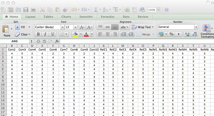
          Ffairad  = gamma3*FSM + gamma5*Frelman + epsilon1,
          Fcsat    = beta2*Ffairad + gamma4*FSM + gamma7*Frelman + epsilon2,
          Fcommit  = beta1*Ffairad + beta3*Fcsat +
                     gamma1*Frelcoll + gamma2*FSM + gamma6*Frelman + epsilon3;
     variance
          Frelcoll FSM Frelman = 3*v__,
          e1-e13 = 13*omega__,
          epsilon1-epsilon3 = 3*psi__;
     cov
          Frelcoll FSM Frelman = 3*c__;
     bounds
          v1-v3 omega01-omega13 psi1-psi3 > 0;

/* Add gamma8 and gamma9. The result will be
   a saturated model latent variable model, and the whole thing will fit as
   well as the measurement model.  */

proc calis  pshort nostand vardef=n;
     title2 'Second model: Saturated latent variable part';
     fitindex on(only) = [chisq df probchi];
     /* Only fit index is LR chisquared test. */
     var commit1 relcoll1 relman1 fairad1 csat1
         commit2 relcoll2 relman2 fairad2 csat2 SM1 SM2 SM3;
     lineqs
          commit1  = Fcommit   + e1,
          commit2  = lambda2*Fcommit   + e2,
          relcoll1 = Frelcoll + e3,
          relcoll2 = lambda4*Frelcoll + e4,
          relman1  = Frelman  + e5,
          relman2  = lambda6*Frelman  + e6,
          fairad1  = Ffairad  + e7,
          fairad2  = lambda8*Ffairad  + e8,
          csat1    = Fcsat    + e9,
          csat2    = lambda10*Fcsat    + e10,
          SM1      = FSM + e11,
          SM2      = lambda12*FSM + e12,
          SM3      = lambda13*FSM + e13,
          Ffairad  = gamma3*FSM + gamma5*Frelman + gamma8*Frelcoll + epsilon1,
          Fcsat    = beta2*Ffairad + gamma4*FSM + gamma7*Frelman +
                     gamma9*Frelcoll + epsilon2,
          Fcommit  = beta1*Ffairad + beta3*Fcsat +
                     gamma1*Frelcoll + gamma2*FSM + gamma6*Frelman + epsilon3;
     variance
          Frelcoll FSM Frelman = 3*v__,
          e1-e13 = 13*omega__,
          epsilon1-epsilon3 = 3*psi__;
     cov
          Frelcoll FSM Frelman = 3*c__;
     bounds
          v1-v3 omega01-omega13 psi1-psi3 > 0;

/* Could start dropping links to build a proposed model. Instead, explore
   gender differences. Begn by looking at correlation matrices.*/

data diverse2;
     set diverse;
     if gender ne .; /* Discard 2 cases where gender is missing. */
proc sort;  /* Sort is needed to split the analysis by a grouping variable. */
     by gender;

proc corr;
     title2 'Correlations separately for men and women';
     by gender;
     var commit relcol relman fairad csat SM;
Fitting a multi-group model by maximum likelihood presents no problems in theory. Just multiply the likelihoods. You don't even need exactly the same variables.
First, it makes sense to test for differences between the unstructured covariance matrices. If there is no evidence that they are different, why model the difference?
/* diversity2.sas */
title 'Diversity study: Test sex differences';

/* Read data directly from Excel spreadsheet */
proc import datafile="/folders/myfolders/431s17/DiversityA.xls" out=HR dbms=xls;
            getnames=yes;
/* Input data file is DiversityA.xls
   Ouput data set is called HR (For Human Resources)
   dbms=xls The input file is an Excel spreadsheet.
            Necessary to read an Excel spreadsheet directly under unix/linux.
            Works in Windows environment too except for Excel 4.0 spreadsheets.
            The xlsx file type is supported, but as of SAS Version 9.3 it's flaky.
            If there are multiple sheets, use sheet="sheet1" or something.
   getnames=yes   Use column names as variable names                  */

proc format;  /* value labels used in data step below */
     value sexfmt  0 = 'Male'   1 = 'Female' ;
     value racefmt 0 = 'White'   1 = 'Visible Minority' ;

data diverse;
     set HR;
     commit1 = sum(of Com1-Com5);
     commit2 = sum(of Com6-Com10);
     commit = commit1+commit2;
     relcoll1 = RelC1+RelC2+RelC3;
     relcoll2 = RelC4+RelC5;
     relcol = relcol1+relcol2;
     relman1  = sum(of RelM1-RelM6);
     relman2  = sum(of RelM7-RelM12);
     relman = relman1+relman2;
     fairad1  = Fair1+Fair2+Fair3;
     fairad2  = Fair4+Fair5+Fair6;
     fairad = fairad1+fairad2;
     csat1    = Sat1+Sat2;
     csat2    = Sat3+Sat4;
     csat = csat1+csat2;
     SM = sm1+sm2+sm3;
     format gender sexfmt.; format VisMinority racefmt.;

/* Need groups to be in separate SAS data tables to fit a multigroup model. */

data boys;
     set diverse;
     if gender=0; /* Select males. */
data girls;
     set diverse;
     if gender=1; /* Select females. */

/* This should fit the same model to both groups and test against the saturated model. */
proc calis pshort nostand pcorr vardef=n;
           /* Could use chicorrect=eqcovmat option for Box's correction. */
     title2 'Test difference between covariance matrices';
     fitindex on(only) = [chisq df probchi];
     group 1 / label='Males' data=boys;
     group 2 / label='Females' data=girls;
     model 1 / group = 1,2; /* Fit same model to both groups */
     var commit1 relcoll1 relman1 fairad1 csat1
         commit2 relcoll2 relman2 fairad2 csat2 SM1 SM2 SM3;
     lineqs; /* No equations */
     variance commit1 relcoll1 relman1 fairad1 csat1
              commit2 relcoll2 relman2 fairad2 csat2 SM1 SM2 SM3 = 13*v__;
     cov      commit1 relcoll1 relman1 fairad1 csat1
              commit2 relcoll2 relman2 fairad2 csat2 SM1 SM2 SM3 = 78*c__;

     /* G2 = 136.7319, df=91, p = 0.0014 */

proc calis pshort nostand pcorr vardef=n covpattern = eqcovmat;
     title2 'Test difference the easy way.';
     fitindex on(only) = [chisq df probchi];
     var commit1 relcoll1 relman1 fairad1 csat1
         commit2 relcoll2 relman2 fairad2 csat2 SM1 SM2 SM3;
     group 1 / label='Males' data=boys;
     group 2 / label='Females' data=girls;
 /* Box's correction was automatically applied -- but G^2 = objective function * n
   = 0.4588320297 * 298 = 136.7319.  */

/* Now compare the measurement models and hope there's no difference. In the
   reduced model, factor loadings and error variances are the same but Phi,
   the covariance matrix of the latent variables, could still be different
   for men and women. This is really a gamble, because re-parameterization
   mixes the latent variable model and the measurement model together. */

proc calis psummary vardef=n; /* Print fit summary only */
     title2 'Full 2-group FA Model: All parameters different for M and F';
     fitindex on(only) = [chisq df probchi];
     /* Only fit index is LR chisquared test. */
     var commit1 relcoll1 relman1 fairad1 csat1
         commit2 relcoll2 relman2 fairad2 csat2 SM1 SM2 SM3;
     group 1 / label='Males' data=boys;
     group 2 / label='Females' data=girls;
      model 1 / group = 1; /* Males: precede parameter names with b */
     lineqs
          commit1  = Fcommit   + e1,
          commit2  = blambda2*Fcommit   + e2,
          relcoll1 = Frelcoll + e3,
          relcoll2 = blambda4*Frelcoll + e4,
          relman1  = Frelman  + e5,
          relman2  = blambda6*Frelman  + e6,
          fairad1  = Ffairad  + e7,
          fairad2  = blambda8*Ffairad  + e8,
          csat1    = Fcsat    + e9,
          csat2    = blambda10*Fcsat    + e10,
          SM1      = FSM + e11,
          SM2      = blambda12*FSM + e12,
          SM3      = blambda13*FSM + e13;
     variance
          Fcommit Frelcoll Frelman Ffairad Fcsat FSM = 6*bv__,
          e1-e13 = 13*bomega__;
     cov
          Fcommit Frelcoll Frelman Ffairad Fcsat FSM = 15*bc__;
     bounds
          bv1-bv6 bomega01-bomega13 > 0;

     model 2 / group = 2; /* Females: precede parameter names with g */
     lineqs
          commit1  = Fcommit   + e1,
          commit2  = glambda2*Fcommit   + e2,
          relcoll1 = Frelcoll + e3,
          relcoll2 = glambda4*Frelcoll + e4,
          relman1  = Frelman  + e5,
          relman2  = glambda6*Frelman  + e6,
          fairad1  = Ffairad  + e7,
          fairad2  = glambda8*Ffairad  + e8,
          csat1    = Fcsat    + e9,
          csat2    = glambda10*Fcsat    + e10,
          SM1      = FSM + e11,
          SM2      = glambda12*FSM + e12,
          SM3      = glambda13*FSM + e13;
     variance
          Fcommit Frelcoll Frelman Ffairad Fcsat FSM = 6*gv__,
          e1-e13 = 13*gomega__;
     cov
          Fcommit Frelcoll Frelman Ffairad Fcsat FSM = 15*gc__;
     bounds
          gv1-gv6 gomega01-gomega13 > 0;


/************************** Reduced model*******************************/
proc calis  psummary vardef=n; /* Print fit summary only */
     title2 'Reduced Model: Factor loadings and measurement error variances equal for M and F';
     fitindex on(only) = [chisq df probchi]; /* Just chi-squared test */
     var commit1 relcoll1 relman1 fairad1 csat1
         commit2 relcoll2 relman2 fairad2 csat2 SM1 SM2 SM3;
     group 1 / label='Males' data=boys;
     group 2 / label='Females' data=girls;
      /* Make lambdas and omegas the same for M and F: Omit b and g */
     model 1 / group = 1; /* Males */
     lineqs
          commit1  = Fcommit   + e1,
          commit2  = lambda2*Fcommit   + e2,
          relcoll1 = Frelcoll + e3,
          relcoll2 = lambda4*Frelcoll + e4,
          relman1  = Frelman  + e5,
          relman2  = lambda6*Frelman  + e6,
          fairad1  = Ffairad  + e7,
          fairad2  = lambda8*Ffairad  + e8,
          csat1    = Fcsat    + e9,
          csat2    = lambda10*Fcsat    + e10,
          SM1      = FSM + e11,
          SM2      = lambda12*FSM + e12,
          SM3      = lambda13*FSM + e13;
     variance
          Fcommit Frelcoll Frelman Ffairad Fcsat FSM = 6*bv__,
          e1-e13 = 13*omega__;
     cov
          Fcommit Frelcoll Frelman Ffairad Fcsat FSM = 15*bc__;
     bounds
          bv1-bv6 omega01-omega13 > 0;

     model 2 / group = 2; /* Females */
     lineqs
          commit1  = Fcommit   + e1,
          commit2  = lambda2*Fcommit   + e2,
          relcoll1 = Frelcoll + e3,
          relcoll2 = lambda4*Frelcoll + e4,
          relman1  = Frelman  + e5,
          relman2  = lambda6*Frelman  + e6,
          fairad1  = Ffairad  + e7,
          fairad2  = lambda8*Ffairad  + e8,
          csat1    = Fcsat    + e9,
          csat2    = lambda10*Fcsat    + e10,
          SM1      = FSM + e11,
          SM2      = lambda12*FSM + e12,
          SM3      = lambda13*FSM + e13;
     variance
          Fcommit Frelcoll Frelman Ffairad Fcsat FSM = 6*gv__,
          /* e1-e13 = 13*omega__;  Automatic naming started with 14 rather than 01 */
          e1-e13 = omega01-omega13; /* Much better. Works up front too. */
     cov
          Fcommit Frelcoll Frelman Ffairad Fcsat FSM = 15*gc__;
     bounds
          gv1-gv6 omega01-omega13 > 0;

proc iml;
     title2 'Likelihood ratio test of H0: Measurement models equal';
     /* 7 lambdas and 13 omegas are equal under H0 */
     Gsq = 149.5559 - 118.1198; pvalue = 1 - probchi(Gsq,20);
     print Gsq pvalue;
Ouch. That's really ambiguous, especially because those suppressed lambdas are propagated throughout the latent variable model, so that part of any difference in the measurement models is absorbed by the latent variable model. Maybe the question should be whether the correlation matrices of the latent variables are different. If not, drop it. If so, consider a classical path analysis of the latent variables.
/* diversity3.sas */
title 'Diversity study: Test sex differences with a standardized latent model';

/* Read data directly from Excel spreadsheet */
proc import datafile="/folders/myfolders/431s17/DiversityA.xls" out=HR dbms=xls;
            getnames=yes;
/* Input data file is DiversityA.xls
   Ouput data set is called HR (For Human Resources)
   dbms=xls The input file is an Excel spreadsheet.
            Necessary to read an Excel spreadsheet directly under unix/linux.
            Works in Windows environment too except for Excel 4.0 spreadsheets.
            The xlsx file type is supported, but as of SAS Version 9.3 it's flaky.
            If there are multiple sheets, use sheet="sheet1" or something.
   getnames=yes   Use column names as variable names                  */

proc format;  /* value labels used in data step below */
     value sexfmt  0 = 'Male'   1 = 'Female' ;
     value racefmt 0 = 'White'   1 = 'Visible Minority' ;

data diverse;
     set HR;
     commit1 = sum(of Com1-Com5);
     commit2 = sum(of Com6-Com10);
     commit = commit1+commit2;
     relcoll1 = RelC1+RelC2+RelC3;
     relcoll2 = RelC4+RelC5;
     relcol = relcol1+relcol2;
     relman1  = sum(of RelM1-RelM6);
     relman2  = sum(of RelM7-RelM12);
     relman = relman1+relman2;
     fairad1  = Fair1+Fair2+Fair3;
     fairad2  = Fair4+Fair5+Fair6;
     fairad = fairad1+fairad2;
     csat1    = Sat1+Sat2;
     csat2    = Sat3+Sat4;
     csat = csat1+csat2;
     SM = sm1+sm2+sm3;
     format gender sexfmt.; format VisMinority racefmt.;

/* First fit combined data for comparison. Match chi-square = 59.7243 */

proc calis vardef=n psummary data=diverse; /* Print fit summary only. */
     title2 'Combined data:  Match fit chi-square = 59.7243';
     fitindex on(only) = [chisq df probchi];
     /* Only fit index is LR chisquared test. */
     var commit1 relcoll1 relman1 fairad1 csat1
         commit2 relcoll2 relman2 fairad2 csat2 SM1 SM2 SM3;
     lineqs
          commit1  = lambda1*Fcommit  + e1,
          commit2  = lambda2*Fcommit  + e2,
          relcoll1 = lambda3*Frelcoll + e3,
          relcoll2 = lambda4*Frelcoll + e4,
          relman1  = lambda5*Frelman  + e5,
          relman2  = lambda6*Frelman  + e6,
          fairad1  = lambda7*Ffairad  + e7,
          fairad2  = lambda8*Ffairad  + e8,
          csat1    = lambda9*Fcsat    + e9,
          csat2    = lambda10*Fcsat    + e10,
          SM1      = lambda11*FSM + e11,
          SM2      = lambda12*FSM + e12,
          SM3      = lambda13*FSM + e13;
     variance
          Fcommit Frelcoll Frelman Ffairad Fcsat FSM = 6*1,
          e1-e13 = omega01-omega13;
     cov
          Fcommit Frelcoll Frelman Ffairad Fcsat FSM = cor01-cor15;
     bounds
          omega01-omega13 > 0;

/* Need groups to be in separate SAS data tables to fit a multigroup model. */

data boys;
     set diverse;
     if gender=0; /* Select males. */
data girls;
     set diverse;
     if gender=1; /* Select females. */

/* Test equality of latent correlation matrices. In the full model, all
   parameters are potentially different for M and F. In the reduced model,
   measurement models may be different but the latent correlation matrices
   are the same. */

proc calis  pshort nostand vardef=n;
     title2 'Full 2-group FA Model: All parameters different for M and F';
     title3 'Compare chisq = 118.1198, df=100, p = 0.1043';
     fitindex on(only) = [chisq df probchi];
     /* Only fit index is LR chisquared test. */
     var commit1 relcoll1 relman1 fairad1 csat1
         commit2 relcoll2 relman2 fairad2 csat2 SM1 SM2 SM3;
     group 1 / label='Males' data=boys;
     group 2 / label='Females' data=girls;
     model 1 / group = 1; /* Males: precede parameter names with b */
     lineqs
          commit1  = blambda1*Fcommit  + e1,
          commit2  = blambda2*Fcommit  + e2,
          relcoll1 = blambda3*Frelcoll + e3,
          relcoll2 = blambda4*Frelcoll + e4,
          relman1  = blambda5*Frelman  + e5,
          relman2  = blambda6*Frelman  + e6,
          fairad1  = blambda7*Ffairad  + e7,
          fairad2  = blambda8*Ffairad  + e8,
          csat1    = blambda9*Fcsat    + e9,
          csat2    = blambda10*Fcsat   + e10,
          SM1      = blambda11*FSM     + e11,
          SM2      = blambda12*FSM     + e12,
          SM3      = blambda13*FSM     + e13;
     variance
          Fcommit Frelcoll Frelman Ffairad Fcsat FSM = 6*1,
          e1-e13 = bomega01-bomega13;
     cov
          Fcommit Frelcoll Frelman Ffairad Fcsat FSM = bc01-bc15;
     bounds
          bomega01-bomega13 > 0;

     model 2 / group = 2; /* Females: precede parameter names with g */
     lineqs
          commit1  = glambda1*Fcommit  + e1,
          commit2  = glambda2*Fcommit  + e2,
          relcoll1 = glambda3*Frelcoll + e3,
          relcoll2 = glambda4*Frelcoll + e4,
          relman1  = glambda5*Frelman  + e5,
          relman2  = glambda6*Frelman  + e6,
          fairad1  = glambda7*Ffairad  + e7,
          fairad2  = glambda8*Ffairad  + e8,
          csat1    = glambda9*Fcsat    + e9,
          csat2    = glambda10*Fcsat   + e10,
          SM1      = glambda11*FSM     + e11,
          SM2      = glambda12*FSM     + e12,
          SM3      = glambda13*FSM     + e13;
     variance
          Fcommit Frelcoll Frelman Ffairad Fcsat FSM = 6*1,
          e1-e13 = gomega01-gomega13;
     cov
          Fcommit Frelcoll Frelman Ffairad Fcsat FSM = gc01-gc15;
     bounds
          gomega01-gomega13 > 0;
     /* Wald tests for sex differences in correlations */
     simtests SexDiffCorr = [FcommitFrelcoll FcommitFrelman  FrelcollFrelman
                             FcommitFfairad  FrelcollFfairad FrelmanFfairad
                             FcommitFcsat    FrelcollFcsat   FrelmanFcsat
                             FfairadFcsat    FcommitFSM      FrelcollFSM
                             FrelmanFSM      FfairadFSM      FcsatFSM];
              FcommitFrelcoll = bc01-gc01;
              FcommitFrelman = bc02-gc02;
              FrelcollFrelman = bc03-gc03;
              FcommitFfairad = bc04-gc04;
              FrelcollFfairad = bc05-gc05;
              FrelmanFfairad = bc06-gc06;
              FcommitFcsat = bc07-gc07;
              FrelcollFcsat = bc08-gc08;
              FrelmanFcsat = bc09-gc09;
              FfairadFcsat = bc10-gc10;
              FcommitFSM = bc11-gc11;
              FrelcollFSM = bc12-gc12;
              FrelmanFSM = bc13-gc13;
              FfairadFSM = bc14-gc14;
              FcsatFSM = bc15-gc15;

/************************** Reduced model*******************************/
proc calis  psummary vardef=n; /* Print fit summary only */
     title2 'Reduced Model: Inter-factor correlations equal for M and F';
     fitindex on(only) = [chisq df probchi]; /* Just chi-squared test */
     var commit1 relcoll1 relman1 fairad1 csat1
         commit2 relcoll2 relman2 fairad2 csat2 SM1 SM2 SM3;
     group 1 / label='Males' data=boys;
     group 2 / label='Females' data=girls;
     /* Inter-factor correlations equal for M and F, but
        measurement models can still be different.        */
      model 1 / group = 1; /* Males: precede some parameter names with b */
     lineqs
          commit1  = blambda1*Fcommit  + e1,
          commit2  = blambda2*Fcommit  + e2,
          relcoll1 = blambda3*Frelcoll + e3,
          relcoll2 = blambda4*Frelcoll + e4,
          relman1  = blambda5*Frelman  + e5,
          relman2  = blambda6*Frelman  + e6,
          fairad1  = blambda7*Ffairad  + e7,
          fairad2  = blambda8*Ffairad  + e8,
          csat1    = blambda9*Fcsat    + e9,
          csat2    = blambda10*Fcsat   + e10,
          SM1      = blambda11*FSM     + e11,
          SM2      = blambda12*FSM     + e12,
          SM3      = blambda13*FSM     + e13;
     variance
          Fcommit Frelcoll Frelman Ffairad Fcsat FSM = 6*1,
          e1-e13 = bomega01-bomega13;
     cov
          Fcommit Frelcoll Frelman Ffairad Fcsat FSM = cor01-cor15;
          /* cor01-cor15 are the same for M and F */
     bounds
          bomega01-bomega13 > 0;

     model 2 / group = 2; /* Females: precede parameter names with g */
     lineqs
          commit1  = glambda1*Fcommit  + e1,
          commit2  = glambda2*Fcommit  + e2,
          relcoll1 = glambda3*Frelcoll + e3,
          relcoll2 = glambda4*Frelcoll + e4,
          relman1  = glambda5*Frelman  + e5,
          relman2  = glambda6*Frelman  + e6,
          fairad1  = glambda7*Ffairad  + e7,
          fairad2  = glambda8*Ffairad  + e8,
          csat1    = glambda9*Fcsat    + e9,
          csat2    = glambda10*Fcsat   + e10,
          SM1      = glambda11*FSM     + e11,
          SM2      = glambda12*FSM     + e12,
          SM3      = glambda13*FSM     + e13;
     variance
          Fcommit Frelcoll Frelman Ffairad Fcsat FSM = 6*1,
          e1-e13 = gomega01-gomega13;
     cov
          Fcommit Frelcoll Frelman Ffairad Fcsat FSM = cor01-cor15;
          /* cor01-cor15 are the same for M and F */
     bounds
          gomega01-gomega13 > 0;

proc iml;
     title2 'Likelihood ratio test of H0: Factor correlations equal for M and F';
     Gsq = 161.6637 - 118.1198; pvalue = 1 - probchi(Gsq,15);
     print Gsq pvalue;
Estimated Latent Correlation Matrices
MALES
            Fcommit   Frelcoll   Frelman   Ffairad   Fcsat   FSM

Fcommit     1.00000
Frelcoll    0.56795   1.00000
Frelman     0.70072   0.74659   1.00000
Ffairad     0.68624   0.65515   0.79499   1.00000
Fcsat       0.55626   0.57492   0.63431   0.74924   1.00000
FSM         0.36390   0.23917   0.38086   0.36494   0.34198   1.00000

FEMALES
            Fcommit   Frelcoll   Frelman   Ffairad   Fcsat   FSM

Fcommit     1.00000
Frelcoll    0.24325   1.00000
Frelman     0.18878   0.36782   1.00000
Ffairad     0.47947   0.41514   0.68970   1.00000
Fcsat       0.43709   0.34585   0.54682   0.73444   1.00000
FSM         0.18913   0.14361   0.15782   0.31197   0.07130   1.00000

It's easy enough to standardize factors, but standardizing a full latent model induces dependence among its parameters. It's best to experiment with a simple example.
/* ClassicalPathExperiment.sas */
title 'Latent path analysis of simulated Fuller Pig data';
title2 'Based on STA431s17 HW 7 Check';

data double;
     infile '/folders/myfolders/431s17/431s17HW7/openpigs.data.txt' firstobs=7; /* Skip first 6 lines */
     input Farm W1 V1 W2 V2;
     label W1 = 'Breeding sows 1'
           W2 = 'Breeding sows 2'
           V1 = 'Births 1'
           V2 = 'Births 2';

proc calis  pshort vardef=n ;
     title3 'Ordinary double measurement for comparison';
     fitindex on(only) = [chisq df probchi];
     /* Only fit index is LR chisquared test. */
     var W1 V1 W2 V2;
     lineqs
          Fbirths  = beta1 Fbreeders + epsilon,
          W1 = Fbreeders + e1,
          V1 = Fbirths   + e2,
          W2 = Fbreeders + e3,
          V2 = Fbirths + e4;
     variance
          Fbreeders = phi, epsilon = psi,
          e1 = omega11, e2 = omega22, e3 = omega33, e4 = omega44;
     cov
          e1 e2 = omega12  , e3 e4 = omega34 ;
     bounds 0.0 < phi psi omega11 omega22 omega33 omega44;

proc calis  psummary vardef=n ;
     title3 'Ordinary reduced model for H0: beta1=0';
     fitindex on(only) = [chisq df probchi];
     /* Only fit index is LR chisquared test. */
     var W1 V1 W2 V2;
     lineqs
          Fbirths  = beta1 Fbreeders + epsilon,
          W1 = Fbreeders + e1,
          V1 = Fbirths   + e2,
          W2 = Fbreeders + e3,
          V2 = Fbirths + e4;
     variance
          Fbreeders = phi, epsilon = psi,
          e1 = omega11, e2 = omega22, e3 = omega33, e4 = omega44;
     cov
          e1 e2 = omega12  , e3 e4 = omega34 ;
     bounds 0.0 < phi psi omega11 omega22 omega33 omega44;
     lincon beta1=0;

proc calis pshort vardef=n ;
     title3 'Standardized Latent Model';
     fitindex on(only) = [chisq df probchi];
     /* Only fit index is LR chisquared test. */
     var W1 V1 W2 V2;
     lineqs
          Fbirths  = beta1 Fbreeders + epsilon,
          W1 = lambdaX*Fbreeders + e1,
          V1 = lambdaY*Fbirths   + e2,
          W2 = lambdaX*Fbreeders + e3,
          V2 = lambdaY*Fbirths   + e4;
     variance
          Fbreeders = 1, epsilon = psi,
          e1 = omega11, e2 = omega22, e3 = omega33, e4 = omega44;
     cov
          e1 e2 = omega12  , e3 e4 = omega34 ;
     bounds 0.0 < omega11 omega22 omega33 omega44,
            -1.0 < beta1 < 1.0; /* To keep psi positive */
     /* SAS programming statements to define dependent parameter
        connection: Var(Y) = Var(beta1 X + epsilon)
                 =>    1   = beta1^2 Var(X) + Var(epsilon)
                           = beta1^2 + psi, so set */
     psi = 1. - beta1*beta1;

proc calis psummary vardef=n ;
     title3 'Standardized Reduced model for testing H0: beta1=0';
     fitindex on(only) = [chisq df probchi];
     /* Only fit index is LR chisquared test. */
     var W1 V1 W2 V2;
     lineqs
          Fbirths  = beta1 Fbreeders + epsilon,
          W1 = lambdaX*Fbreeders + e1,
          V1 = lambdaY*Fbirths   + e2,
          W2 = lambdaX*Fbreeders + e3,
          V2 = lambdaY*Fbirths   + e4;
     variance
          Fbreeders = 1, epsilon = psi,
          e1 = omega11, e2 = omega22, e3 = omega33, e4 = omega44;
     cov
          e1 e2 = omega12  , e3 e4 = omega34 ;
     bounds 0.0 < omega11 omega22 omega33 omega44,
            -1.0 < beta1 < 1.0; /* To keep psi positive */
     lincon beta1=0;
     /* SAS programming statements to define dependent parameter
        connection: Var(Y) = Var(beta1 X + epsilon)
                 =>    1   = beta1^2 Var(X) + Var(epsilon)
                           = beta1^2 + psi, so set */
     psi = 1. - beta1*beta1;
Likelihood ratio tests are invariant to parameterization, while Wald tests are not.
Ordinary double measurement
     Chi-square         = 0.0871
     beta1-hat          = 0.75667
     t stat             = 14.0472
     stand beta1-hat    = 0.92669
     stand t            = 34.9896
     Full-reduced chisq = 44.5280 - 0.0871 = 44.4409

Standardized latent model
     Chi-square         = 0.0871
     beta1-hat          = 0.92669
     t stat             = 34.9895
     stand beta1-hat    = 0.92669
     stand t            = 34.9895
     Full-reduced chisq = 44.5278 - 0.0871 = 44.4407